When the data is spewing garbage
I spent the last couple of months analyzing data from sensors, surveys, and logs. No matter how many charts I created, how well sophisticated the algorithms are, the results are always misleading.
Throwing a random forest at the data is the same as injecting it with a virus. A virus that has no intention other than hurting your insights as if your data is spewing garbage.
Even worse, when you show your new findings to the CEO, and Oops guess what? He/she found a flaw, something that doesn’t smell right, your discoveries don’t match their understanding about the domain — After all, they are domain experts who know better than you, you as an analyst or a developer.
Right away, the blood rushed into your face, your hands are shaken, a moment of silence, followed by, probably, an apology.
That’s not bad at all. What if your findings were taken as a guarantee, and your company ended up making a decision based on them?.
You ingested a bunch of dirty data, didn’t clean it up, and you told your company to do something with these results that turn out to be wrong. You’re going to be in a lot of trouble!.
Incorrect or inconsistent data leads to false conclusions. And so, how well you clean and understand the data has a high impact on the quality of the results.
Two real examples were given on Wikipedia.
For instance, the government may want to analyze population census figures to decide which regions require further spending and investment on infrastructure and services. In this case, it will be important to have access to reliable data to avoid erroneous fiscal decisions.
In the business world, incorrect data can be costly. Many companies use customer information databases that record data like contact information, addresses, and preferences. For instance, if the addresses are inconsistent, the company will suffer the cost of resending mail or even losing customers.
In fact, a simple algorithm can outweigh a complex one just because it was given enough and high-quality data.
For these reasons, it was important to have a step-by-step guideline, a cheat sheet, that walks through the quality checks to be applied.
But first, what’s the thing we are trying to achieve?. What does it mean quality data?. What are the measures of quality data?. Understanding what are you trying to accomplish, your ultimate goal is critical prior to taking any actions.
Frankly speaking, I couldn’t find a better explanation for the quality criteria other than the one on Wikipedia. So, I am going to summarize it here.
The degree to which the data conform to defined business rules or constraints.
Data-Type Constraints: values in a particular column must be of a particular datatype, e.g., boolean, numeric, date, etc.Range Constraints: typically, numbers or dates should fall within a certain range.Mandatory Constraints: certain columns cannot be empty.Unique Constraints: a field, or a combination of fields, must be unique across a dataset.Set-Membership constraints: values of a column come from a set of discrete values, e.g. enum values. For example, a person’s gender may be male or female.Foreign-key constraints: as in relational databases, a foreign key column can’t have a value that does not exist in the referenced primary key.Regular expression patterns: text fields that have to be in a certain pattern. For example, phone numbers may be required to have the pattern(999) 999–9999.Cross-field validation: certain conditions that span across multiple fields must hold. For example, a patient’s date of discharge from the hospital cannot be earlier than the date of admission.
The degree to which the data is close to the true values.
While defining all possible valid values allows invalid values to be easily spotted, it does not mean that they are accurate.
A valid street address mightn’t actually exist. A valid person’s eye colour, say blue, might be valid, but not true (doesn’t represent the reality).
Another thing to note is the difference between accuracy and precision. Saying that you live on the earth is, actually true. But, not precise. Where on the earth?. Saying that you live at a particular street address is more precise.
The degree to which all required data is known.
Missing data is going to happen for various reasons. One can mitigate this problem by questioning the original source if possible, say re-interviewing the subject.
Chances are, the subject is either going to give a different answer or will be hard to reach again.
The degree to which the data is consistent, within the same data set or across multiple data sets.
Inconsistency occurs when two values in the data set contradict each other.
A valid age, say 10, mightn’t match with the marital status, say divorced. A customer is recorded in two different tables with two different addresses.
Which one is true?.
The degree to which the data is specified using the same unit of measure.
The weight may be recorded either in pounds or kilos. The date might follow the USA format or European format. The currency is sometimes in USD and sometimes in YEN.
And so data must be converted to a single measure unit.
The workflow is a sequence of three steps aiming at producing high-quality data and taking into account all the criteria we’ve talked about.
Inspection: Detect unexpected, incorrect, and inconsistent data.Cleaning: Fix or remove the anomalies discovered.Verifying: After cleaning, the results are inspected to verify correctness.Reporting: A report about the changes made and the quality of the currently stored data is recorded.
What you see as a sequential process is, in fact, an iterative, endless process. One can go from verifying to inspection when new flaws are detected.
Inspecting the data is time-consuming and requires using many methods for exploring the underlying data for error detection. Here are some of them:
A summary statistics about the data, called data profiling, is really helpful to give a general idea about the quality of the data.
For example, check whether a particular column conforms to particular standards or pattern. Is the data column recorded as a string or number?.
How many values are missing?. How many unique values in a column, and their distribution?. Is this data set is linked to or have a relationship with another?.
By analyzing and visualizing the data using statistical methods such as mean, standard deviation, range, or quantiles, one can find values that are unexpected and thus erroneous.
For example, by visualizing the average income across the countries, one might see there are some outliers (link has an image). Some countries have people who earn much more than anyone else. Those outliers are worth investigating and are not necessarily incorrect data.
Several software packages or libraries available at your language will let you specify constraints and check the data for violation of these constraints.
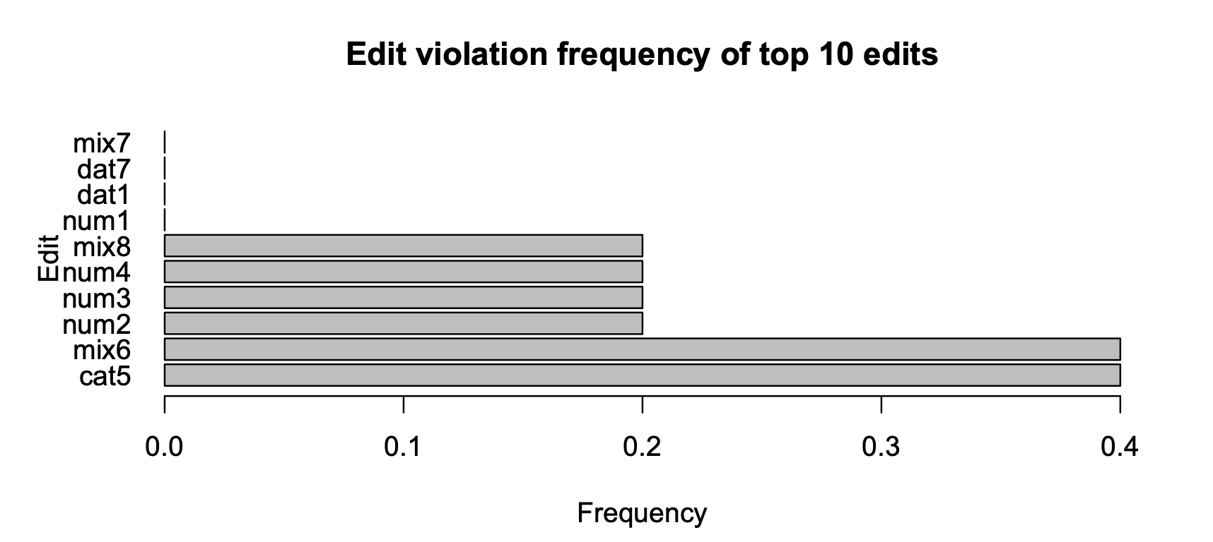
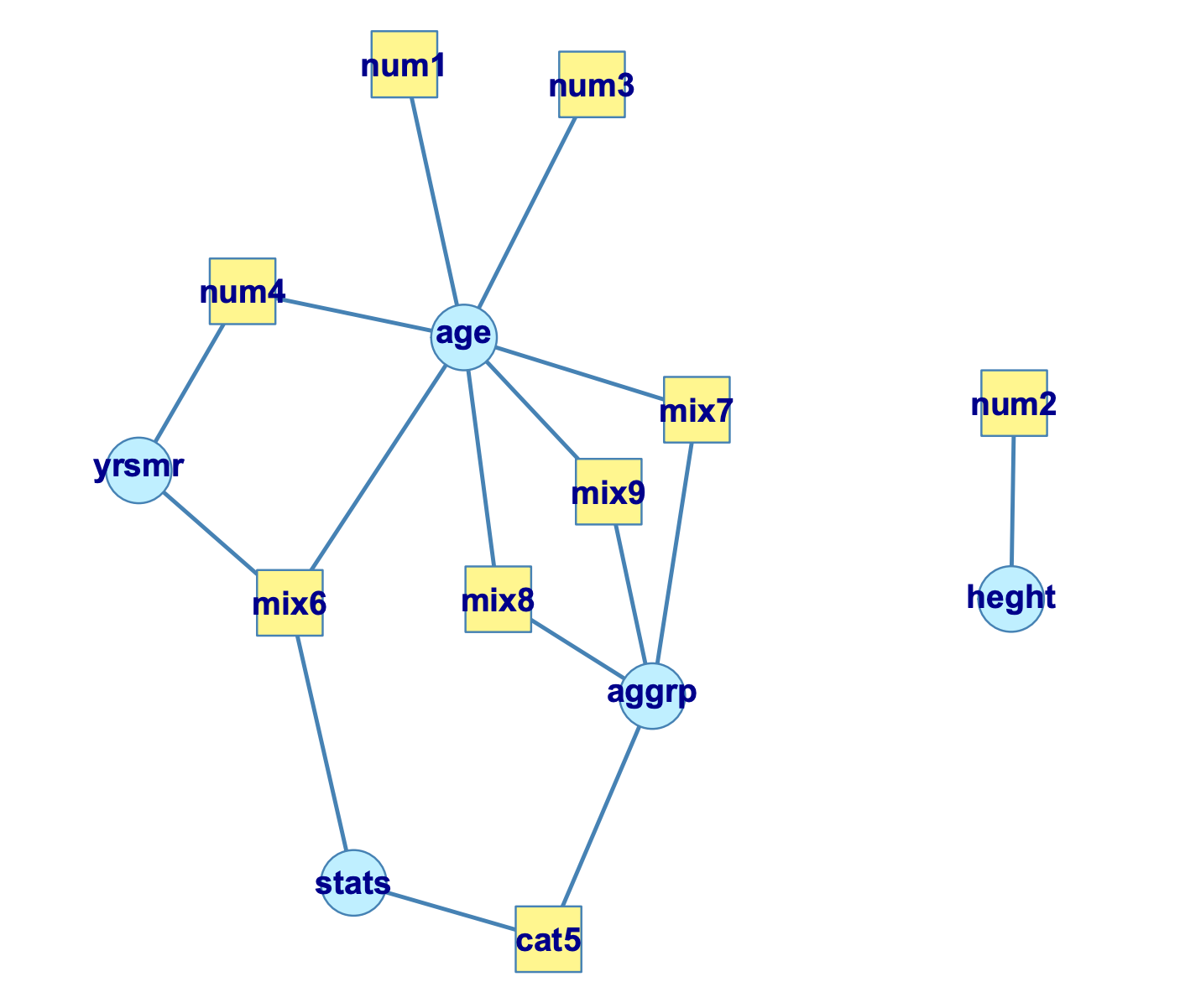
Moreover, they can not only generate a report of which rules were violated and how many times but also create a graph of which columns are associated with which rules.
The age, for example, can’t be negative, and so the height. Other rules may involve multiple columns in the same row, or across datasets.
Data cleaning involve different techniques based on the problem and the data type. Different methods can be applied with each has its own trade-offs.
Overall, incorrect data is either removed, corrected, or imputed.
Irrelevant data are those that are not actually needed, and don’t fit under the context of the problem we’re trying to solve.
For example, if we were analyzing data about the general health of the population, the phone number wouldn’t be necessary — column-wise.
Similarly, if you were interested in only one particular country, you wouldn’t want to include all other countries. Or, study only those patients who went to the surgery, we wouldn’t include everyone — row-wise.
Only if you are sure that a piece of data is unimportant, you may drop it. Otherwise, explore the correlation matrix between feature variables.
And even though you noticed no correlation, you should ask someone who is domain expert. You never know, a feature that seems irrelevant, could be very relevant from a domain perspective such as a clinical perspective.
Duplicates are data points that are repeated in your dataset.
It often happens when for example
- Data are combined from different sources
- The user may hit submit button twice thinking the form wasn’t actually submitted.
- A request to online booking was submitted twice correcting wrong information that was entered accidentally in the first time.
A common symptom is when two users have the same identity number. Or, the same article was scrapped twice.
And therefore, they simply should be removed.
Make sure numbers are stored as numerical data types. A date should be stored as a date object, or a Unix timestamp (number of seconds), and so on.
Categorical values can be converted into and from numbers if needed.
This is can be spotted quickly by taking a peek over the data types of each column in the summary (we’ve discussed above).
A word of caution is that the values that can’t be converted to the specified type should be converted to NA value (or any), with a warning being displayed. This indicates the value is incorrect and must be fixed.
Remove white spaces: Extra white spaces at the beginning or the end of a string should be removed.
" hello world " => "hello world
Pad strings: Strings can be padded with spaces or other characters to a certain width. For example, some numerical codes are often represented with prepending zeros to ensure they always have the same number of digits.
313 => 000313 (6 digits)
Fix typos: Strings can be entered in many different ways, and no wonder, can have mistakes.
Gender
m
Male
fem.
FemalE
Femle
This categorical variable is considered to have 5 different classes, and not 2 as expected: male and female since each value is different.
A bar plot is useful to visualize all the unique values. One can notice some values are different but do mean the same thing i.e. “information_technology” and “IT”. Or, perhaps, the difference is just in the capitalization i.e. “other” and “Other”.
Therefore, our duty is to recognize from the above data whether each value is male or female. How can we do that?.
The first solution is to manually map each value to either “male” or “female”.
dataframe['gender'].map({'m': 'male', fem.': 'female', ...})
The second solution is to use pattern match. For example, we can look for the occurrence of m or M in the gender at the beginning of the string.
re.sub(r"\^m\$", 'Male', 'male', flags=re.IGNORECASE)
The third solution is to use fuzzy matching: An algorithm that identifies the distance between the expected string(s) and each of the given one. Its basic implementation counts how many operations are needed to turn one string into another.
Gender   male  female
m         3      5
Male      1      3
fem.      5      3
FemalE    3      2
Femle     3      1
Furthermore, if you have a variable like a city name, where you suspect typos or similar strings should be treated the same. For example, “lisbon” can be entered as “lisboa”, “lisbona”, “Lisbon”, etc.
City     Distance from "lisbon"
lisbon       0
lisboa       1
Lisbon       1
lisbona      2
london       3
...
If so, then we should replace all values that mean the same thing to one unique value. In this case, replace the first 4 strings with “lisbon”.
Watch out for values like “0”, “Not Applicable”, “NA”, “None”, “Null”, or “INF”, they might mean the same thing: The value is missing.
Our duty is to not only recognize the typos but also put each value in the same standardized format.
For strings, make sure all values are either in lower or upper case.
For numerical values, make sure all values have a certain measurement unit.
The hight, for example, can be in meters and centimetres. The difference of 1 meter is considered the same as the difference of 1 centimetre. So, the task here is to convert the heights to one single unit.
For dates, the USA version is not the same as the European version. Recording the date as a timestamp (a number of milliseconds) is not the same as recording the date as a date object.
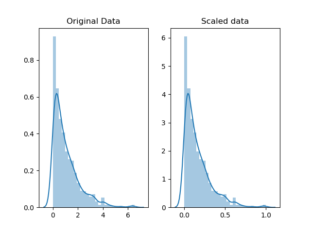
Scaling means to transform your data so that it fits within a specific scale, such as 0–100 or 0–1.
For example, exam scores of a student can be re-scaled to be percentages (0–100) instead of GPA (0–5).
It can also help in making certain types of data easier to plot. For example, we might want to reduce skewness to assist in plotting (when having such many outliers). The most commonly used functions are log, square root, and inverse.
Scaling can also take place on data that has different measurement units.
Student scores on different exams say, SAT and ACT, can’t be compared since these two exams are on a different scale. The difference of 1 SAT score is considered the same as the difference of 1 ACT score. In this case, we need re-scale SAT and ACT scores to take numbers, say, between 0–1.
By scaling, we can plot and compare different scores.
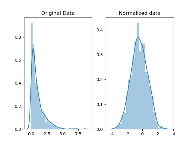
While normalization also rescales the values into a range of 0–1, the intention here is to transform the data so that it is normally distributed. Why?
In most cases, we normalize the data if we’re going to be using statistical methods that rely on normally distributed data. How?
One can use the log function, or perhaps, use one of these methods.
Depending on the scaling method used, the shape of the data distribution might change. For example, the “Standard Z score” and “Student’s t-statistic” (given in the link above) preserve the shape, while the log function mighn’t.
Normalization vs Scaling (using Feature scaling) — source
Given the fact the missing values are unavoidable leaves us with the question of what to do when we encounter them. Ignoring the missing data is the same as digging holes in a boat; It will sink.
There are three, or perhaps more, ways to deal with them.
If the missing values in a column rarely happen and occur at random, then the easiest and most forward solution is to drop observations (rows) that have missing values.
If most of the column’s values are missing, and occur at random, then a typical decision is to drop the whole column.
This is particularly useful when doing statistical analysis, since filling in the missing values may yield unexpected or biased results.
It means to calculate the missing value based on other observations. There are quite a lot of methods to do that.
Firstone is usingstatistical valueslike mean, median. However, none of these guarantees unbiased data, especially if there are many missing values.
Mean is most useful when the original data is not skewed, while the median is more robust, not sensitive to outliers, and thus used when data is skewed.
In a normally distributed data, one can get all the values that are within 2 standard deviations from the mean. Next, fill in the missing values by generating random numbers between (mean — 2 * std) & (mean + 2 * std)
rand = np.random.randint(average_age - 2*std_age, average_age + 2*std_age, size = count_nan_age)dataframe["age"][np.isnan(dataframe["age"])] = rand
Second. Using alinear regression. Based on the existing data, one can calculate the best fit line between two variables, say, house price vs. size m².
It is worth mentioning that linear regression models are sensitive to outliers.
Third.Hot-deck: Copying values from other similar records. This is only useful if you have enough available data. And, it can be applied to numerical and categorical data.
One can take the random approach where we fill in the missing value with a random value. Taking this approach one step further, one can first divide the dataset into two groups (strata), based on some characteristic, say gender, and then fill in the missing values for different genders separately, at random.
In sequential hot-deck imputation, the column containing missing values is sorted according to auxiliary variable(s) so that records that have similar auxiliaries occur sequentially. Next, each missing value is filled in with the value of the first following available record.
What is more interesting is that 𝑘 nearest neighbour imputation, which classifies similar records and put them together, can also be utilized. A missing value is then filled out by finding first the 𝑘 records closest to the record with missing values. Next, a value is chosen from (or computed out of) the 𝑘 nearest neighbours. In the case of computing, statistical methods like mean (as discussed before) can be used.
Some argue that filling in the missing values leads to a loss in information, no matter what imputation method we used.
That’s because saying that the data is missing is informative in itself, and the algorithm should know about it. Otherwise, we’re just reinforcing the pattern already exist by other features.
This is particularly important when the missing data doesn’t happen at random. Take for example a conducted survey where most people from a specific race refuse to answer a certain question.
Missing numeric data can be filled in with say, 0, but has these zeros must be ignored when calculating any statistical value or plotting the distribution.
While categorical data can be filled in with say, “Missing”: A new category which tells that this piece of data is missing.
Missing values are not the same as default values. For instance, zero can be interpreted as either missing or default, but not both.
Missing values are not “unknown”. A conducted research where some people didn’t remember whether they have been bullied or not at the school, should be treated and labelled as unknown and not missing.
Every time we drop or impute values we are losing information. So, flagging might come to the rescue.
They are values that are significantly different from all other observations. Any data value that lies more than (1.5 * IQR) away from the Q1 and Q3 quartiles is considered an outlier.
Outliers are innocent until proven guilty. With that being said, they should not be removed unless there is a good reason for that.
For example, one can notice some weird, suspicious values that are unlikely to happen, and so decides to remove them. Though, they worth investigating before removing.
It is also worth mentioning that some models, like linear regression, are very sensitive to outliers. In other words, outliers might throw the model off from where most of the data lie.
These errors result from having two or more values in the same row or across datasets that contradict with each other.
For example, if we have a dataset about the cost of living in cities. The total column must be equivalent to the sum of rent, transport, and food.
city       rent  transportation food  total
libson     500        20         40    560
paris      750        40         60    850
Similarly, a child can’t be married. An employee’s salary can’t be less than the calculated taxes.
The same idea applies to related data across different datasets.
When done, one should verify correctness by re-inspecting the data and making sure it rules and constraints do hold.
For example, after filling out the missing data, they might violate any of the rules and constraints.
It might involve some manual correction if not possible otherwise.
Reporting how healthy the data is, is equally important to cleaning.
As mentioned before, software packages or libraries can generate reports of the changes made, which rules were violated, and how many times.
In addition to logging the violations, the causes of these errors should be considered. Why did they happen in the first place?.
If you made it that far, I am happy you were able to hold until the end. But, None of what mentioned is valuable without embracing the quality culture.
No matter how robust and strong the validation and cleaning process is, one will continue to suffer as new data come in.
It is better to guard yourself against a disease instead of spending the time and effort to remedy it.
These questions help to evaluate and improve the data quality:
How the data is collected, and under what conditions.
The environment where the data was collected does matter. The environment includes, but not limited to, the location, timing, weather conditions, etc.
Questioning subjects about their opinion regarding whatever while they are on their way to work is not the same as while they are at home. Patients under a study who have difficulties using the tablets to answer a questionnaire might throw off the results.
What does the data represent?.
Does it include everyone? Only the people in the city?. Or, perhaps, only those who opted to answer because they had a strong opinion about the topic.
What are the methods used to clean the data and why?.
Different methods can be better in different situations or with different data types.
Do you invest the time and money in improving the process?.
Investing in people and the process is as critical as investing in the technology.
And finally, … it doesn’t go without saying,
Thank you for reading!


