CellPyLib is a library for working with Cellular Automata, for Python. Currently, only 1- and 2-dimensional k-color cellular automata with periodic boundary conditions are supported. The size of the neighbourhood can be adjusted. The cellular automata produced by this library match the corresponding cellular automata available at atlas.wolfram.com.
Example usage:
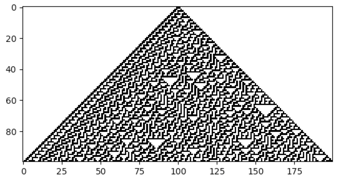
import cellpylib as cpl

# initialize a CA with 200 cells (a random initialization is also available)
cellular_automaton = cpl.init_simple(200)

# evolve the CA for 100 time steps, using Rule 30 as defined in NKS
cellular_automaton = cpl.evolve(cellular_automaton, timesteps=100,
                                apply_rule=lambda n, c, t: cpl.nks_rule(n, 30))

# plot the resulting CA evolution
cpl.plot(cellular_automaton)CellPyLib can be installed via pip:
pip install cellpylib
Requirements for using this library are Python 3.5.3, numpy 1.14.0, and matplotlib 2.0.2.
The size of the cell neighbourhood can be varied by setting the parameter r when calling the evolve function. The
value of r represents the number of cells to the left and to the right of the cell under consideration. Thus, to
get a neighbourhood size of 3, r should be 1, and to get a neighbourhood size of 7, r should be 3.
As an example, consider the work of M. Mitchell et al., carried out in the 1990s, involving the creation (discovery) of
a cellular automaton that solves the density classification problem: if the initial random binary vector contains
more than 50% of 1s, then a cellular automaton that solves this problem will give rise to a vector that contains only
1s after a fixed number of time steps, and likewise for the case of 0s. A very effective cellular automaton that solves
this problem most of the time was found using a Genetic Algorithm.
import cellpylib as cpl

cellular_automaton = cpl.init_random(149)

# Mitchell et al. discovered this rule using a Genetic Algorithm
rule_number = 6667021275756174439087127638698866559

# evolve the CA, setting r to 3, for a neighbourhood size of 7
cellular_automaton = cpl.evolve(cellular_automaton, timesteps=149,
                                apply_rule=lambda n, c, t: cpl.binary_rule(n, rule_number), r=3)

cpl.plot(cellular_automaton)
For more information, see:
Melanie Mitchell, James P. Crutchfield, and Rajarshi Das, "Evolving Cellular Automata with Genetic Algorithms: A Review of Recent Work", In Proceedings of the First International Conference on Evolutionary Computation and Its Applications (EvCA'96), Russian Academy of Sciences (1996).
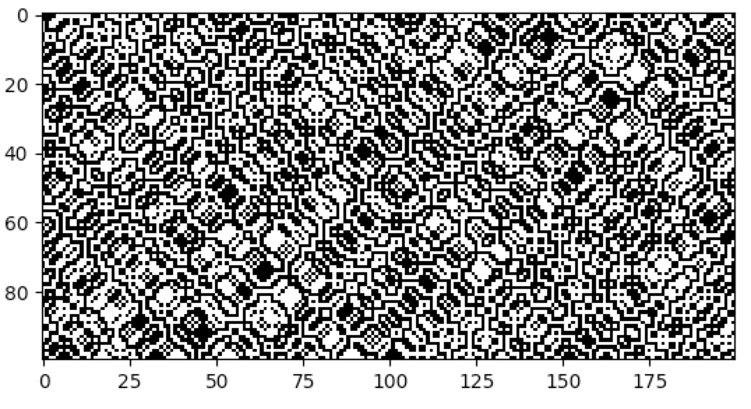
The number of states, or colors, that a cell can adopt is given by k. For example, a binary cellular automaton, in which a cell can
assume only values of 0 and 1, has k = 2. CellPyLib supports any value of k. A built-in function, totalistic_rule,
is an implementation of the Totalistic cellular automaton rule,
as described in Wolfram's NKS. The code snippet below illustrates using this rule.
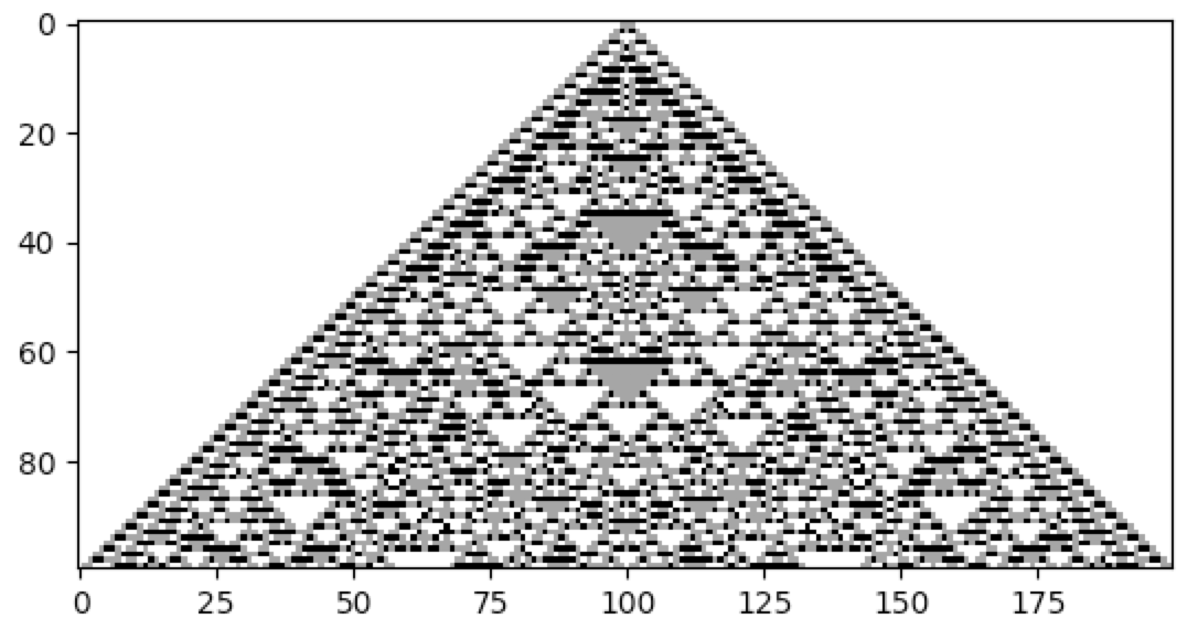
A value of k of 3 is used, but any value between (and including) 2 and 36 is currently supported. The rule number is
given in base 10 but is interpreted as the rule in base k (thus rule 777 corresponds to '1001210' when k = 3).
import cellpylib as cpl

cellular_automaton = cpl.init_simple(200)

# evolve the CA, using totalistic rule 777 for a 3-color CA
cellular_automaton = cpl.evolve(cellular_automaton, timesteps=100,
                                apply_rule=lambda n, c, t: cpl.totalistic_rule(n, k=3, rule=777))

cpl.plot(cellular_automaton)One way to specify cellular automata rules is with rule tables. Rule tables are enumerations of all possible neighbourhood states together with their cell state mappings. For any given neighbourhood state, a rule table provides the associated cell state value. CellPyLib provides a built-in function for creating random rule tables. The following snippet demonstrates its usage:
import cellpylib as cpl

rule_table, actual_lambda, quiescent_state = cpl.random_rule_table(lambda_val=0.45, k=4, r=2,
                                                                   strong_quiescence=True, isotropic=True)

cellular_automaton = cpl.init_random(128, k=4)

# use the built-in table_rule to use the generated rule table
cellular_automaton = cpl.evolve(cellular_automaton, timesteps=200,
                                apply_rule=lambda n, c, t: cpl.table_rule(n, rule_table), r=2)
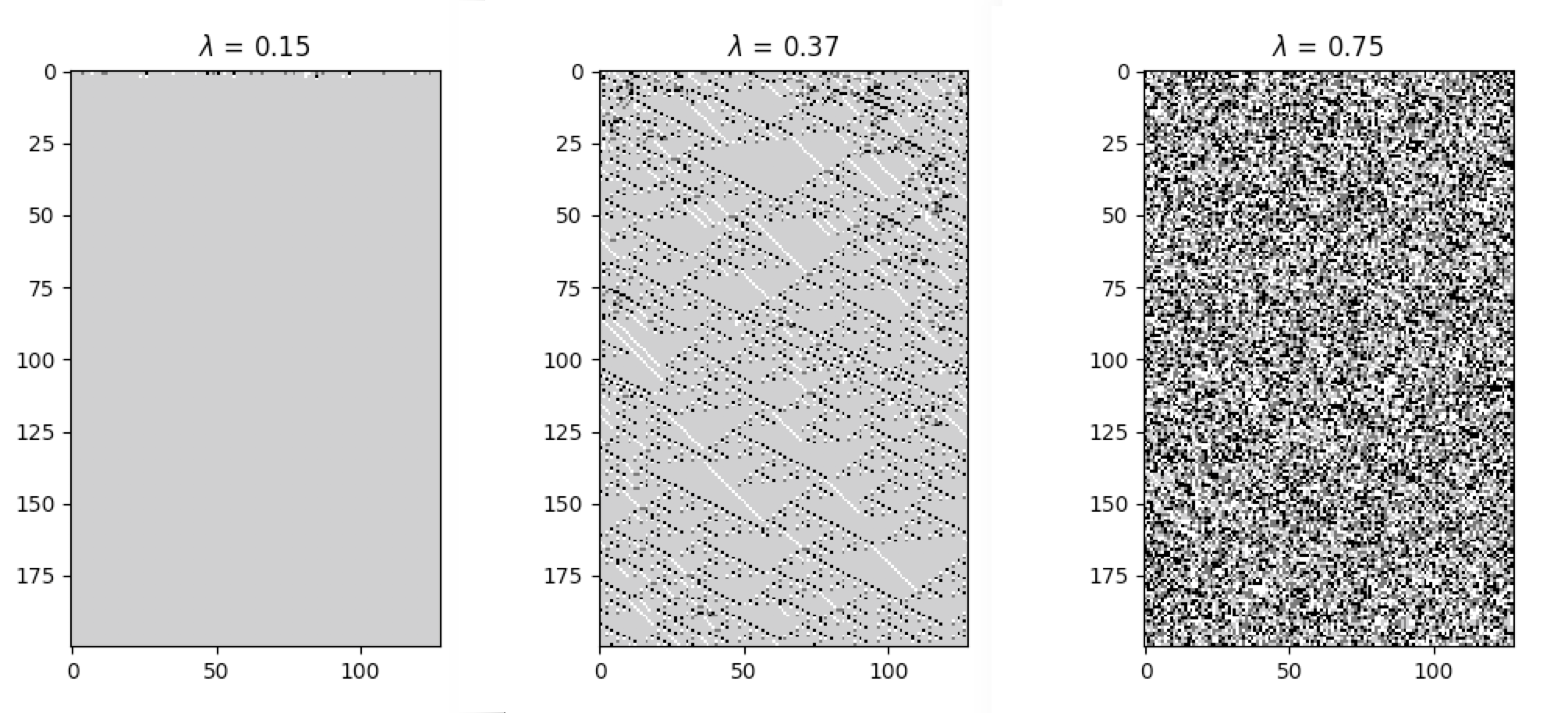
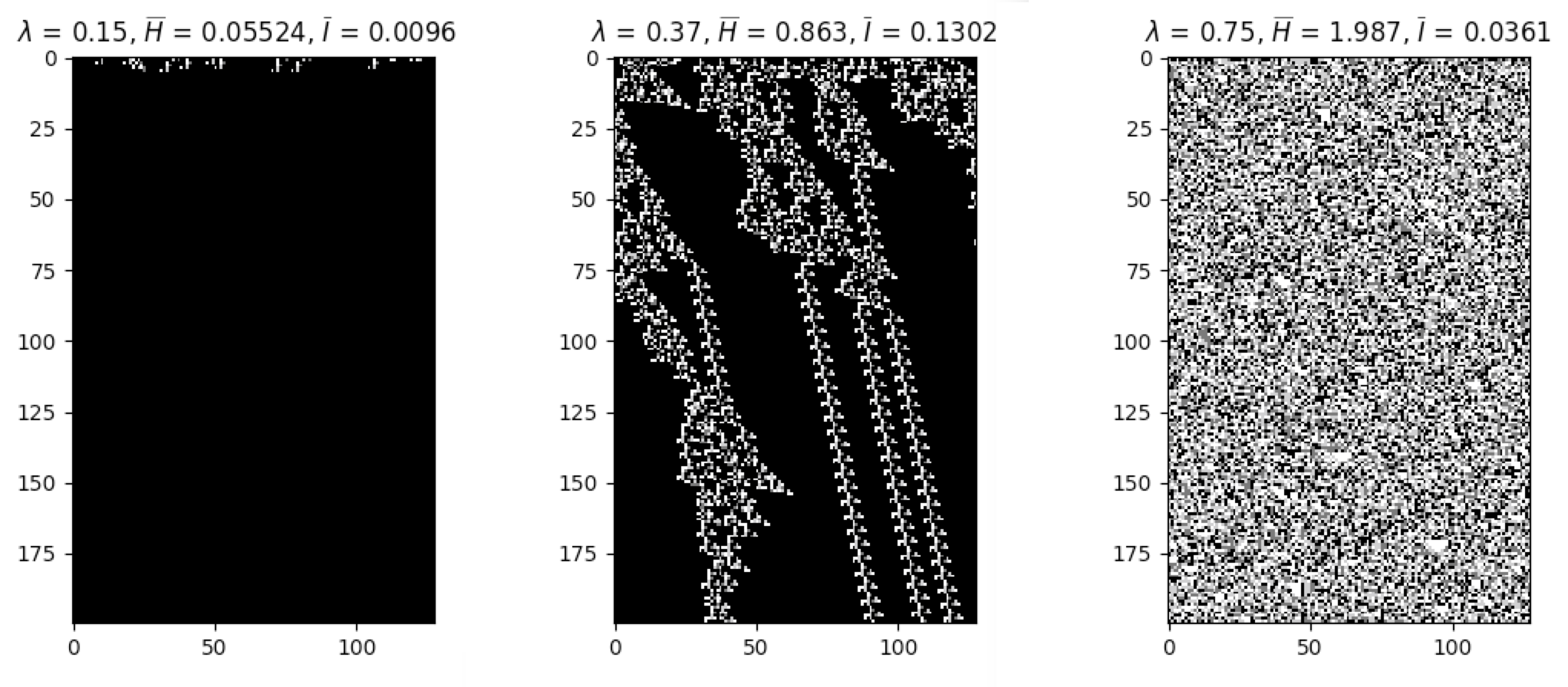
The following plots demonstrate the effect of varying the lambda parameter:
C. G. Langton describes the lambda parameter, and the transition from order to criticality to chaos in cellular automata while varying the lambda parameter, in the paper:
Langton, C. G. (1990). Computation at the edge of chaos: phase transitions and emergent computation. Physica D: Nonlinear Phenomena, 42(1-3), 12-37.
CellPyLib provides various built-in functions which can act as measures of complexity in the cellular automata being examined.
Average cell entropy can reveal something about the presence of information within cellular automata dynamics. The
built-in function average_cell_entropy provides the average Shannon entropy per single cell in a given cellular
automaton. The following snippet demonstrates the calculation of the average cell entropy:
import cellpylib as cpl

cellular_automaton = cpl.init_random(200)

cellular_automaton = cpl.evolve(cellular_automaton, timesteps=1000,
                                apply_rule=lambda n, c, t: cpl.nks_rule(n, 30))

# calculate the average cell entropy; the value will be ~0.999 in this case
avg_cell_entropy = cpl.average_cell_entropy(cellular_automaton)
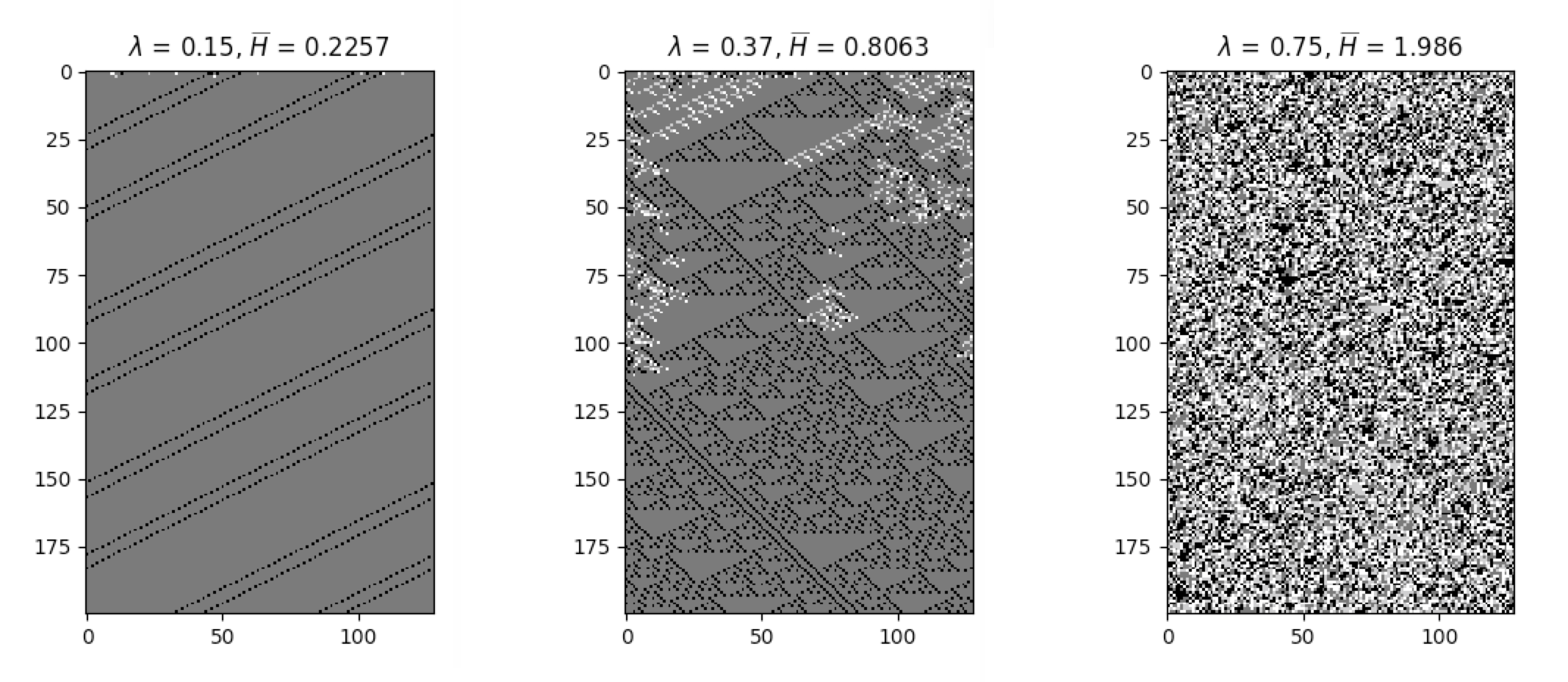
The following plots illustrate how average cell entropy changes as a function of lambda:
The degree to which a cell state is correlated to its state in the next time step can be described using mutual
information. Ideal levels of correlation are required for effective processing of information. The built-in function
average_mutual_information provides the average mutual information between a cell and itself in the next time step
(the temporal distance can be adjusted). The following snippet demonstrates the calculation of the average mutual
information:
import cellpylib as cpl

cellular_automaton = cpl.init_random(200)

cellular_automaton = cpl.evolve(cellular_automaton, timesteps=1000,
                                apply_rule=lambda n, c, t: cpl.nks_rule(n, 30))

# calculate the average mutual information between a cell and itself in the next time step
avg_mutual_information = cpl.average_mutual_information(cellular_automaton)
The following plots illustrate how average mutual information changes as a function of lambda:
Elementary cellular automata can be explicitly made to be reversible. The following example demonstrates the creation of the elementary reversible cellular automaton rule 90R:
import cellpylib as cpl

cellular_automaton = cpl.init_random(200)
r = cpl.ReversibleRule(cellular_automaton[0], 90)

cellular_automaton = cpl.evolve(cellular_automaton, timesteps=100,
                                apply_rule=r.apply_rule)

cpl.plot(cellular_automaton)In addition to discrete values, cellular automata can assume continuous values. CellPyLib supports
continuous-valued automata. To create cellular automata with continuous values--or any kind of data type--simply
specify the dtype parameter when invoking any of the init and evolve built-in functions. For example, to create
a cellular automata with continuous values, one might specify the following parameter: dtype=np.float32.
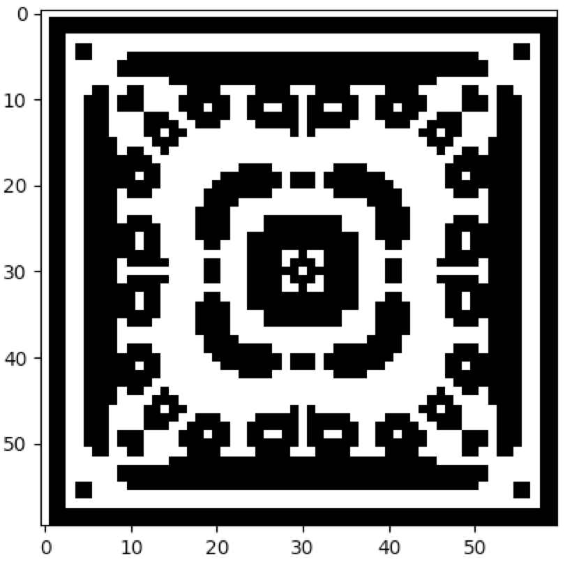
CellPyLib supports 2-dimensional cellular automata with periodic boundary conditions. The number of states, k, can be any whole number. The neighbourhood radius, r, can also be any whole number, and both Moore and von Neumann neighbourhood types are supported. The following snippet demonstrates creating a 2D totalistic cellular automaton:
import cellpylib as cpl

# initialize a 60x60 2D cellular automaton
cellular_automaton = cpl.init_simple2d(60, 60)

# evolve the cellular automaton for 30 time steps,
#  applying totalistic rule 126 to each cell with a Moore neighbourhood
cellular_automaton = cpl.evolve2d(cellular_automaton, timesteps=30, neighbourhood='Moore',
                                  apply_rule=lambda n, c, t: cpl.totalistic_rule(n, k=2, rule=126))

cpl.plot2d(cellular_automaton)
The plot2d function plots the state of the cellular automaton at the final time step:
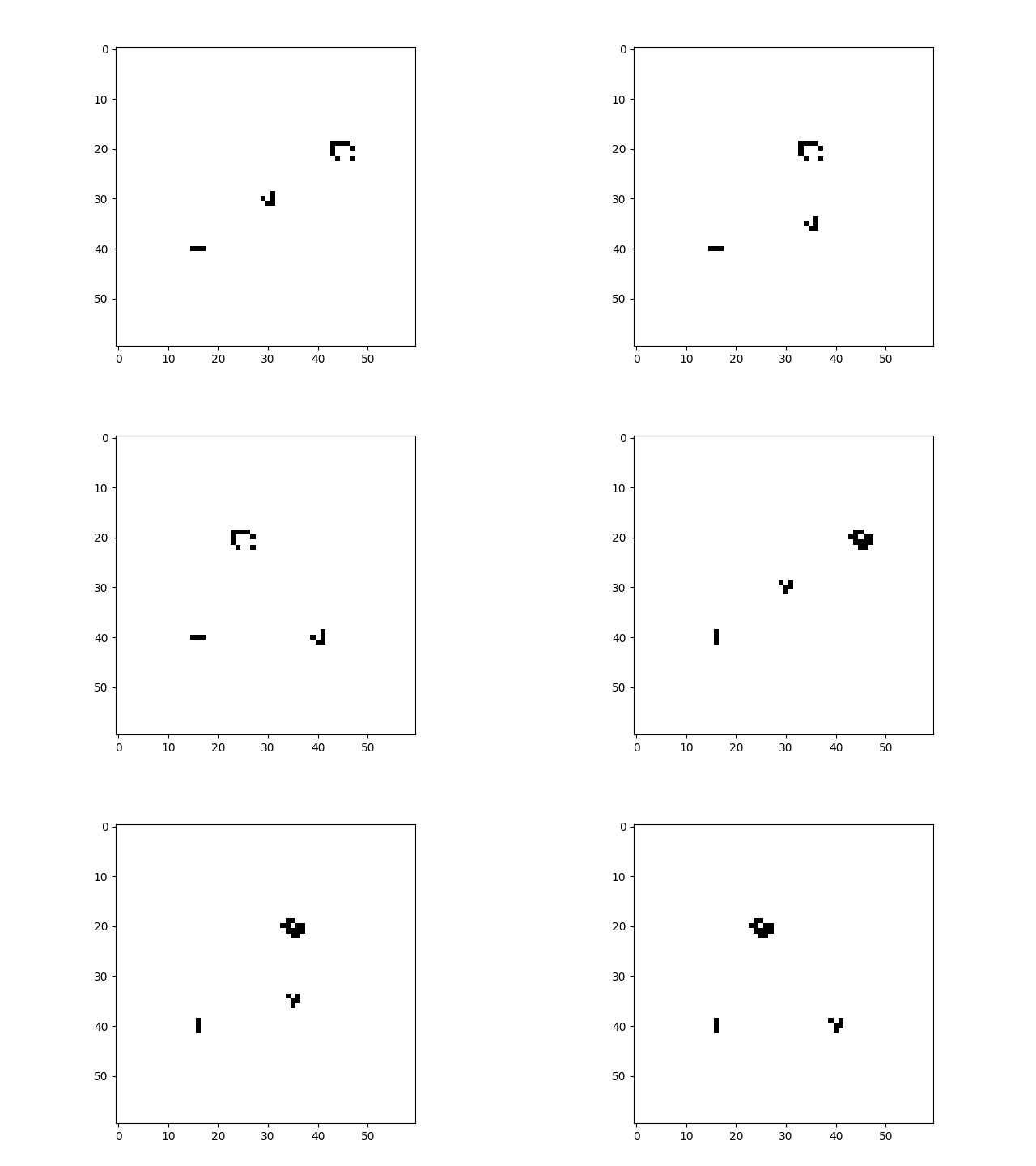
There are a number of built-in plotting functions for 2D cellular automata. For example, plot2d_animate will animate
the evolution of the cellular automaton. This is illustrated in the following snippet, which demonstrates the built-in
Game of Life rule:
import cellpylib as cpl

# Glider
cellular_automaton = cpl.init_simple2d(60, 60)
cellular_automaton[:, [28,29,30,30], [30,31,29,31]] = 1

# Blinker
cellular_automaton[:, [40,40,40], [15,16,17]] = 1

# Light Weight Space Ship (LWSS)
cellular_automaton[:, [18,18,19,20,21,21,21,21,20], [45,48,44,44,44,45,46,47,48]] = 1

# evolve the cellular automaton for 60 time steps
cellular_automaton = cpl.evolve2d(cellular_automaton, timesteps=60, neighbourhood='Moore',
                                  apply_rule=cpl.game_of_life_rule)

cpl.plot2d_animate(cellular_automaton)
For more information about Conway's Game of Life, see:
Conway, J. (1970). The game of life. Scientific American, 223(4), 4.
This project has been published on Zenodo, which provides a DOI, as well as an easy way to generate citations in a number of formats. For example, this project may be cited as:
Antunes, Luis M. (2019, March 10). CellPyLib: A Python Library for working with Cellular Automata. Zenodo. http://doi.org/10.5281/zenodo.3893115
BibTeX:
@software{antunes_luis_m_2019_3893115,
  author       = {Antunes, Luis M.},
  title        = {{CellPyLib: A Python Library for working with
                   Cellular Automata}},
  month        = mar,
  year         = 2019,
  publisher    = {Zenodo},
  doi          = {10.5281/zenodo.3893115},
  url          = {https://doi.org/10.5281/zenodo.3893115}
}
Please star this repository if you find it useful, or use it as part of your research.
Copyright (c) 2018-2020 Luis M. Antunes (@lantunes) All rights reserved.
